Support Vector Machines (SVMs)

SVMs are a powerful class of supervised machines learning algorithms for both classification and regression problems. In the context of classification, they can be viewed as maximum margin linear classifiers. Why? Well, we’ll see that in a bit

The SVM uses an objective which explicitly encourages lower out-of-sample error (good generalization performance).

For the first part we will assume that the two classes are linearly separable. For non-linear boundaries, we will see that we project the data points into higher dimension so that they can be separated linearly using a plane.

import numpy as np
import matplotlib.pyplot as plt
%matplotlib inline
from scipy import stats

#for advanced plot styling
import seaborn as sns; sns.set()

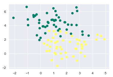
Let’s create a dataset of two classes and let the classes be linearly separable for now.

Linearly separable classes:

from sklearn.datasets.samples_generator import make_blobs

X,y = make_blobs(n_samples=50, centers=2, random_state=0, cluster_std=0.60)
plt.scatter(X[:, 0], X[:, 1], c=y, cmap='summer');

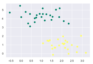
Now, we know that we can differentiate these two classes by drawing a line (decision boundary) between them. But we need to find the optimum decision boundary which will give us the minimum in-sample error.

Many possible separators:

xfit = np.linspace(-1,3.5)
plt.scatter(X[:, 0],X[:, 1], c=y, s=50, cmap='summer')
plt.plot([0.6], [2.1], 'x', color='green', markeredgewidth=2, markersize=10)

# Even though we can plot infinite lines, we will plot 3 lines 
for m, b in [(1, 0.65), (0.5, 1.6), (-0.2, 2.9)]: # m = slope, b = bias, the tuples are the co-ordinates of the lines
    yfit = m*xfit+b
    plt.plot(xfit, yfit, '-k') # '-k' is used to color the lines 'black'

plt.xlim(-1, 3.5);

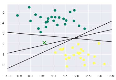
Considering these 3 decision boundaries, the point ‘x’ can easily be misclassified by these decision boundaries. Therefore we want our classifier to be robust to these kind of perturbations in the input that can lead to drastic change in the output. We will see how SVM will overcome this situation by plotting margins.

We know that we can draw millions of lines or decision boundaries for classifying the classes but we want the best decision boundary which have good generalization performance and lowest out-of-sample error. For achieving this what SVM does is instead of having a zero width line, as we have in the above graph, it draws a margin on both the sides of the line of finite length upto the nearest point.

Plotting the margins:

xfit = np.linspace(-1,3.5)
plt.scatter(X[:, 0],X[:, 1], c=y, s=50, cmap='summer')
plt.plot([0.6], [2.1], 'x', color='green', markeredgewidth=2, markersize=10)

# Even though we can plot infinite lines, we will plot 3 lines 
for m, b, d in [(1, 0.65, 0.33), (0.5, 1.6, 0.55), (-0.2, 2.9, 0.2)]: # m = slope, b = bias, the tuples are the co-ordinates of the lines
    yfit = m*xfit+b
    plt.plot(xfit, yfit, '-k') # '-k' is used to color the lines 'black'
    plt.fill_between(xfit, yfit - d, yfit + d, edgecolor = 'none', color = '#AAAAAA', alpha = 0.4) # alpha is for transparency

plt.xlim(-1, 3.5);

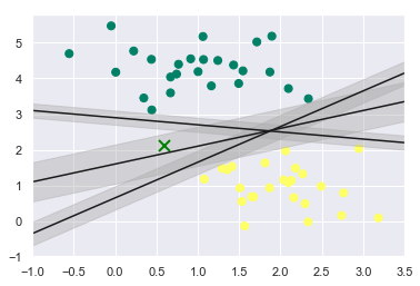
What SVM does is it chooses the decision boundary which has the maximum margin and chooses it as the optimum model.

SVM in practice:

Now that we have a good understanding of when to use SVM, let’s see how to implement SVM from scratch using scikit-learn.

from sklearn.svm import SVC # Support Vector Classifier
model = SVC(kernel='linear', C=1E10)
'''Here C is a hyper parameter that decides how much classification error is allowed. If C is large means the margins are hard
margins meaning that very few or none of the data points will be allowed to creep into the margin space. If C is small means 
the margins are soft margins and some of the data points may be allowed to creep into the margin space. You need to experiment
with this value of C to allow your model to fit the data better.'''
model.fit(X,y)

SVC(C=10000000000.0, break_ties=False, cache_size=200, class_weight=None,
    coef0=0.0, decision_function_shape='ovr', degree=3, gamma='scale',
    kernel='linear', max_iter=-1, probability=False, random_state=None,
    shrinking=True, tol=0.001, verbose=False)

This does not seem to be very intuitive. So let’s plot the decision boundaries.

Plotting the SVM Decision Boundaries:

def plt_decision_boundaries(model, ax=None, plot_support=True):
    if ax is None:
        ax = plt.gca()
    xlim = ax.get_xlim()
    ylim = ax.get_ylim()
    
    # create a gris to evaluate the model
    x = np.linspace(xlim[0], xlim[1], 30)
    y = np.linspace(ylim[0], ylim[1], 30)
    
    Y, X = np.meshgrid(y, x)
    ''' The numpy.meshgrid function is used to create a rectangular grid out of two given one-dimensional arrays representing 
    the Cartesian indexing or Matrix indexing. It returns two 2-Dimensional arrays  representing the X and Y coordinates of 
    all the points.'''
    
    xy = np.vstack([X.ravel(), Y.ravel()]).T
    '''numpy. vstack() function is used to stack the sequence of input arrays vertically to make a single array.'''
    
    P = model.decision_function(xy).reshape(X.shape)
    
    # Plotting decision boundaries and margins
    ax.contour(X, Y, P, colors='k',
               levels=[-1, 0, 1], alpha=0.5,
               linestyles=['--', '-', '--'])
    
    # Plotting the Support Vectors
    '''Support Vectors are the vectors that define the hyperplane. These are the data points that are closest to the margins 
    of the decision boundary. The margins of the decision boundaries are formed as a result of these Support Vectors.'''
    if plot_support:
        ax.scatter(model.support_vectors_[:, 0],
                   model.support_vectors_[:, 1],
                   s=300, linewidth=1, facecolors='none');
    
    ax.set_xlim(xlim)
    ax.set_ylim(ylim)
    
plt.scatter(X[:, 0], X[:, 1], c=y, s=50, cmap='summer')
plt_decision_boundaries(model);

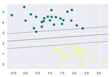
The dotted lines here are known as Margins. The data points touching these margins are known as Support Vectors. In Scikit-Learn, the identity of these points are stored in the support_vectors_ attribute of the Support Vector Classifier.

model.support_vectors_

array([[0.44359863, 3.11530945],
       [2.33812285, 3.43116792],
       [2.06156753, 1.96918596]])

Overlapping classes:

The data points of the two classes that we have seen in the above example were very clearly separable i.e. there was no overlap between the data points of the two classes. But what if there is an overlap between the points of the two classes?

X, y = make_blobs(n_samples=100, centers=2, random_state=0, cluster_std=1.2)
plt.scatter(X[:, 0], X[:, 1], c=y, s=50, cmap='summer');

In order to handle such cases, we need to tune the hyperparameter C of the SVC model. This process of tuning the hyperparameters of a model for a better fit is usually known as Hyperparameter Tuning. Depending upon the value of C, we can have soft or hard margins which decides how much classification error is permittable.

We will now see how changing the value of C affects the fit of our model.

X, y = make_blobs(n_samples=100, centers=2, random_state=0, cluster_std=0.8)

fig, ax = plt.subplots(1, 2, figsize=(16, 6))
fig.subplots_adjust(left=0.0625, right=0.95, wspace=0.1)

for axi, C in zip(ax, [10.0, 0.1]):
    model = SVC(kernel='linear', C=C).fit(X, y)
    axi.scatter(X[:, 0], X[:, 1], c=y, s=50, cmap='autumn')
    plt_decision_boundaries(model, axi)
    axi.scatter(model.support_vectors_[:, 0],
                model.support_vectors_[:, 1],
                s=300, lw=1, facecolors='none');
    axi.set_title('C = {0:.1f}'.format(C), size=14)

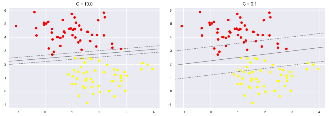
As you can see in the first figure where C=10, very less or none of the data points were allowed to enter into the margin space which is not the case in the second figure where the value of C=0.1.

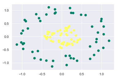
Non-Linearly separable classes:

Till now in our discussion we have seen data that is linearly separable. But what if the data points of the classes are not linearly separable? What if it is something like this:

from sklearn.datasets.samples_generator import make_circles
X, y = make_circles(100, factor=0.3, noise=0.1)

plt.scatter(X[:, 0], X[:, 1], c=y, s=50, cmap='summer')

<matplotlib.collections.PathCollection at 0x24fc9c3d988>

Let’s see what happens if we try to fit the SVC model with kernel as linear:

from sklearn.datasets.samples_generator import make_circles
X, y = make_circles(100, factor=0.3, noise=0.1)

plt.scatter(X[:, 0], X[:, 1], c=y, s=50, cmap='summer')

model = SVC(kernel='linear').fit(X, y)
plt_decision_boundaries(model, plot_support=False);

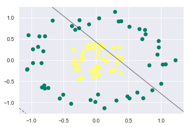
This doesn’t seem to be good, right? Our linear SVC model is not able to differentiate at all between the classes.

Remember at the beginning we discussed in short that if the classes are not linearly we would project the data to higher dimension and then draw a hyperplane that would separate the classes? Lets visualize the data in 3D since we have only 2 classes.

r = np.exp(-(X ** 2).sum(1))

from mpl_toolkits import mplot3d
from ipywidgets import interact, fixed

def plot_3D(elev=30, azim=30, X=X, y=y):
    ax = plt.subplot(projection='3d')
    ax.scatter3D(X[:, 0], X[:, 1], r, c=y, s=50, cmap='summer')
    ax.view_init(elev=elev, azim=azim)
    ax.set_xlabel('x')
    ax.set_ylabel('y')
    ax.set_zlabel('r')

interact(plot_3D, elev=[-150, 150], azip=(-150, 150), X=fixed(X), y=fixed(y));

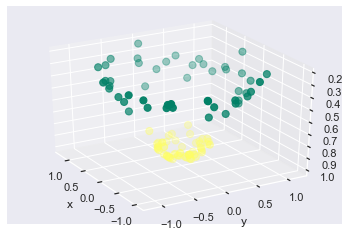
When we project the data to higher dimensions we see that the data becomes linearly separable and we can separate the data using a hyperplane.

But there is one problem here. We had only two classes here so projecting to 3D was no problem but what if there were N classes? We have to project it to N+1 dimensions which is not feasible.

Thanks to SVM, we can overcome this by using the kernel hyperparameter. Using what is called as the kernel trick we can separate the classes without projecting the data to higher dimensions. We just need to change the kernel from Linear to RBF (Radial Basis Function).

model = SVC(kernel='rbf', C=10)
model.fit(X, y)

SVC(C=10, break_ties=False, cache_size=200, class_weight=None, coef0=0.0,
    decision_function_shape='ovr', degree=3, gamma='scale', kernel='rbf',
    max_iter=-1, probability=False, random_state=None, shrinking=True,
    tol=0.001, verbose=False)

Let’s plot the decision boundaries.

plt.scatter(X[:, 0], X[:, 1], c=y, s=50, cmap='summer')
plt_decision_boundaries(model)
plt.scatter(model.support_vectors_[:, 0], model.support_vectors_[:, 1], s=300, lw=1, facecolors='none');

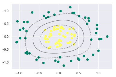
Isn’t it powerful and intuitive!

In this section we have tried to understand and implement how SVM works for both linear and non-linear data. Try implementing it with different set of data points.

Hope you understood and liked this post. If you have any suggestions or any feedback please do reach out to me. I’ll be happy to hear from you.

Will see you in the next post. Till then take care, stay safe and stay healthy!