Deep Residual Learning for Image Recognition (ResNet)

In this section we will try to understand some basic concepts related to ResNet architecture, why is it better than VGG Net, its working and its advantages.

Before trying to understand what ResNet is, first lets try to understand in short what is VGG Net and why ResNet is better than VGG Net.

Understanding VGG Net (VGG 16):

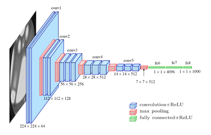
VGG stands for Visual Geometry Group at Oxford University. It was developed by Simonyan and Zisserman for the ILSVRC (Image Net Large Scale Visual Recognition Challenge) 2014 competition. It consists if 16 weight layers (13 Convolution layers and 3 Fully Connected layers) with only 3x3 feature detectors or filters. The error percentage for this architecture was around 7%.

The concept behind VGG net is similar to that of Alexnet, meaning that, as the depth of the network increases, we would increase the number of feature maps or the convolutions. In short, as we go deeper into the network, the number of feature maps increases, so the network becomes wider. There are in total 138 million parameters.

The VGG 16 network architecture is as shown below:

Source: https://www.researchgate.net/figure/Fig-A1-The-standard-VGG-16-network-architecture-as-proposed-in-32-Note-that-only_fig3_322512435

Problem with VGG Net and why do we need ResNets:

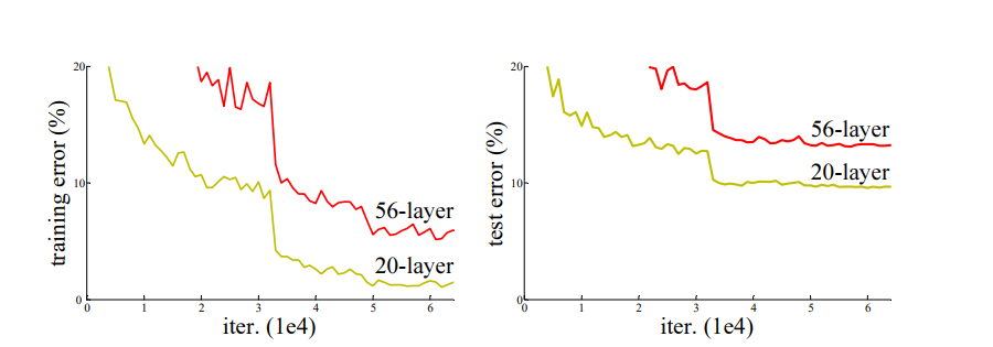
But there was a problem with this architecture. There are a number of layers in this architecture and hence a large number of parameters. This increases complexity of the model. Also as the depth of the neural network increases, accuracy gets saturated and then after a point starts degrading rapidly. This degradation, unexpectedly, is not caused by overfitting. Adding more and more layers to these deep models leads to higher training errors as being tested during experiments mentioned in the paper Deep Residual Learning for Image Recognition.

So, in short, as we add more layers to our deep neural networks, the training error increases. This can be understood using the image below:

Another problem was that of Vanishing Gradient.

So, what is Vanishing Gradient? Well, as we keep on adding more layers to our neural network using some activation function, the gradients of the loss function tends to approach to zero which effectively prevents the weight from changing its value and hence making the network hard to train. During the backpropagation stage, the error is calculated and gradient values are determined. The gradients are sent back to hidden layers and the weights are updated accordingly. This process is continued until the input layer is reached. The gradient becomes smaller and smaller as it reaches the input layer. Therefore, the weights of the initial layers will either update very slowly or remain the same. In other words, the initial layers of the network won’t learn effectively. Hence, the deep neural network will find it difficult to converge and this will hamper the accuracy of the model and hence the training error increases. This problem was largely addressed by normalized initialization i.e. normalizing the initial weights of the networks and Batch Normalization.

Batch Normalization:

It is a technique for training very deep neural networks that standardizes the inputs to a layer for each mini-batch. This has the effect of stabilizing the learning process and dramatically reducing the number of training epochs required to train deep networks. This method allows us to be less careful about initialization.

Didn’t get it yet? Let’s try to understand it in a different way…

It can also be defined as a technique to standardize the inputs to a network, applied to either the activations of a prior layer or inputs directly. In this method we ensure that the pre-activation at each layer are unit gaussians. That is we standardize the input by subtracting with mean and dividing by the standard deviation so that we are making it zero mean and unit variance. So we will have this distribution at each layer of out network. So now at every batch data is coming from a same distribution even if it was of different distant distribution. So how do we compute this mean and variance. The answer lies in the topic itself ‘Batch Normalization’ i.e. we take mean and variance of the current batch and perform standardization.

With batch normalization, we can be confident that the distributions of our activations across hidden layers are reasonably similar. If this is true, then we know that the gradients should have a wider distribution, and not be nearly all zero.

But still we have the degradation problem. We need to overcome this, right? Yes, of course! And that is the reason we are using Deep Residual Learning framework.

Weight Initialization:

Training Deep Neural Networks is complicated by the fact that the distribution of each layer’s inputs changes during training, as the parameters of the previous layers change. This slows down the training by requiring lower learning rates and careful parameter initialization, and makes it notoriously hard to train models with saturating nonlinearities.

The weights that we initialize at the start while training a deep neural network plays an important role in how efficiently our network will be trained and how accurate it would be. Weights should not be initialized to zero because there is no source of asymmetry between neurons if their weights are initialized to be the same. And this is not acceptable. So we will take a look at two of the most popular Weight Initialization (Xavier and He et.al) techniques:

1. Xavier/Glarot Initialization:

   Xavier initialization initializes the weights in the network by drawing them from a distribution with zero mean and a specific variance. It is generally used with tanh activation.

   

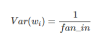
where, fan_in is the number of inputs.

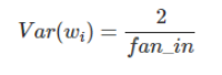
2. He Initialization:

   This is similar to Xavier initialization with a factor multiplies by 2. In order to attain global minimum of the cost function more faster and efficiently, the weights are initialized keeping in mind the size of the previous layer. This results in controlled initialization and as result faster and more efficient gradient descent.

   

Now that we have had a brief overview of what VGG net is and what problem it faces, we will move forward to understand what exactly is ResNet and how does it work.

Residual Networks (ResNet):

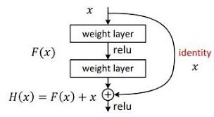
​ Figure1: Residual Block

Residual Networks or ResNet is the same as the conventional deep neural networks with layers such as convolution, activation function or ReLU, pooling and fully connected networks. But the only difference here is that we are adding an identity connection or identity mapping between the layers.

But wait! What is Identity Mapping? You might be knowing of an Identity Matrix, I, which contains only 1’s on the diagonal position starting from the top left corner and 0’s on all other positions. This matrix when multiplied with any other matrix, suppose A, will give the same matrix such that AI = A. The same is happening here, applying identity mapping to the input will give you the output which is the same as the input.

But what is the use of this Identity Mapping? Well, it enables backpropagation signal to reach from output (last) layers to input (first) layers. This is where the whole working of a Residual Neural Network takes place as compared to the conventional Convolutional Neural Network.

As seen in Figure1, F(x) is the Residual Function or the Residual Mapping which is between two convolutional (weight) layers and can be said as the difference between the input (x) and the output (H(x)) of the residual block as shown in Figure1. So, the Residual Function F(x) can be written as:

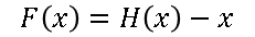
​ Residual Function

So,the main point of introducing this function is that, instead of expecting the stacked layers to learn the approximate the function H(x), which we do in normal stacked convolutional neural network, we let the layers to approximate the residual function F(x). What this means is that, while training the deep residual network, our main aim would be to learn the residual function F(x) which would increase the overall accuracy of the network.

How does the Residual Function help in increasing the accuracy of the network?

Well, we know that during back propagation in a normal stacked deep neural network, as we go to the input layer, the gradients tend to become zero and hence there is no update happening in the weights and hence the network doesn’t learn the weights. And we know what this condition is called, right? Yes, Vanishing Gradient problem.

But when we use the residual function, even if the gradients tend to become zero i.e. even if H(x) becomes zero, the network will atleast learn x (since F(x) = H(x) - x) i.e. it saves the gradients from vanishing. As a result of this, the gradients reach the input layers and the weights are updated which helps the network to learn better and hence accuracy of the network increases. Interesting… isn’t it?

ResNet Architecture

Now, let us look at the ResNet-34 architecture:

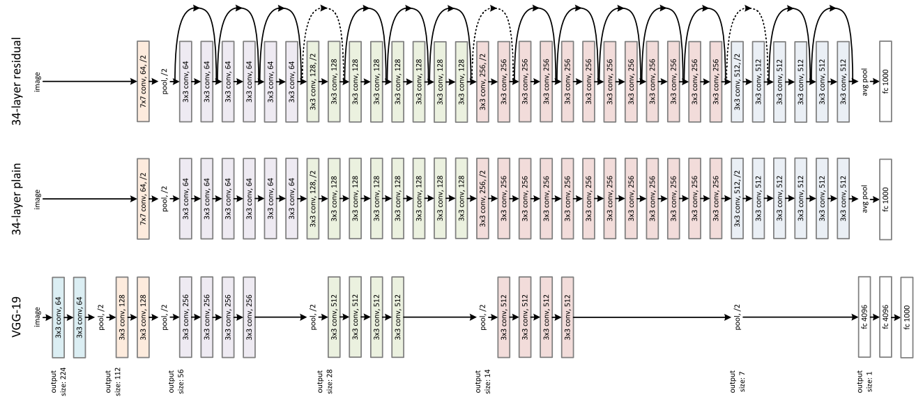
Comparison of VGG-19, 34 layer plain neural network and 34-layer deep residual neural network

The dotted lines indicate change in the size of the image from one residual block to another and is Linear Projection which can be accomplished by using 1x1 kernels.

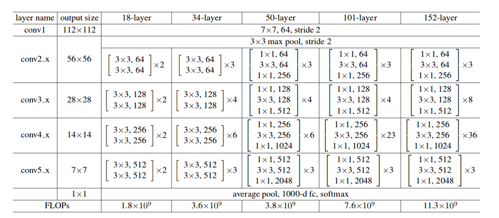
​ Various Deep Residual Network architectures

Advantages of Residual Networks:

As experimented on ImageNet and CIFAR-10 dataset.

1. Easy to optimize
2. Training error does not increase as the depth of the neural network increases as in case of plain neural networks where we just keep on stacking layers.
3. Addition of identity mapping does not introduce any extra parameters. Hence, the computational complexity does not increase.
4. The accuracy gains are higher as the depth increases thus producing results substantially better than other previous networks such as VGG net.

In order to get more clear understanding of the implementation of ResNet and how it works practically, you can visit my github profile where I have deployed ResNet-18 model which is trained on CIFAR-10 dataset.

References:

https://www.quora.com/What-is-the-vanishing-gradient-problem

https://arxiv.org/pdf/1512.03385.pdf

[https://cv-tricks.com/keras/understand-implement-resnets/](